Hill Climbing in Artificial Intelligence

Hill Climbing is a heuristic search algorithm used to find an optimal or near-optimal solution by repeatedly moving from the current state to a better neighboring state based on an evaluation function.

• Used to solve various optimization and search problems in AI.
• Improves the current solution by making small changes and evaluating them.
• Its simple logic makes it easy to implement and adapt to different problems.

Visual Representation

The following diagram illustrates the state space and the corresponding objective function values encountered during hill climbing.

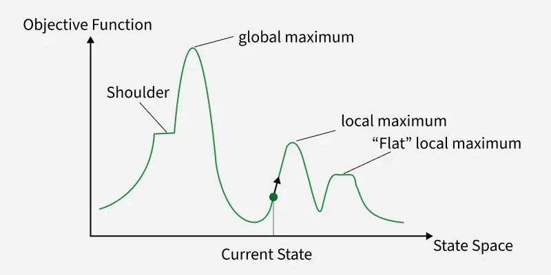
In the state-space diagram:

• X-axis: Represents possible states or configurations in the search space.
• Y-axis: Represents the objective function value corresponding to each state.

The highest point represents the global maximum, which is the optimal solution for a maximization problem.

Key Regions

1. Local Maximum: A state better than its neighbors but not the best overall.
2. Global Maximum: The best state in the state-space diagram where the objective function achieves its highest value.
3. Plateau/Flat Local Maximum: A flat region where neighboring states have the same objective function value.
4. Ridge: A higher region with a slope which can look like a peak.
5. Current State: The algorithm's position in the state-space diagram during its search for the optimal solution.
6. Shoulder: A plateau with an uphill edge allowing the algorithm to move toward better solutions if it continues searching beyond the plateau.

Working

Hill climbing follows these steps:

1. Initial State: Start with an arbitrary or random solution.
2. Neighboring States: Identify neighboring states of the current solution by making small adjustments (mutations or tweaks).
3. Move to a Better State: If one of the neighboring states offers a better evaluation value, move to this new state.
4. Termination: Repeat this process until no neighboring state is better than the current one. At this point, we have reached a local maximum or minimum.

Types

1. Simple Hill Climbing Algorithm: A straightforward variant of hill climbing where the algorithm evaluates each neighboring node one by one and selects the first node that offers an improvement over the current one.

2. Steepest-Ascent Hill Climbing: An enhanced version of simple hill climbing. Instead of moving to the first neighboring node that improves the state, it evaluates all neighbors and moves to the one offering the highest improvement (steepest ascent).

3. Stochastic Hill Climbing: Introduces randomness into the search process. Instead of evaluating all neighbors or selecting the first improvement, it selects a random neighboring node and decides whether to move based on its improvement over the current state.

Features

1. Variant of Generating and Testing Algorithm: Hill Climbing is a specific variant of the generating and testing algorithms. It generates possible solutions, evaluates them and iteratively improves the current solution.

• Generating possible solutions: The algorithm creates potential neighboring solutions.
• Testing solutions: Each generated solution is evaluated.
• Iteration: If a satisfactory solution is found, the algorithm terminates; otherwise returns to the generation step.

2. Greedy Approach: Hill Climbing algorithm uses greedy approach, meaning that at each step it makes the best immediate move based on the evaluation function without considering future states.

Implementation

Step 1: Import libraries

Numpy is used for easy array (vector) manipulation and mathematical operations.

import numpy as np

Hill Climbing is applied to a simple 1-D function where each state has two neighboring solutions.

Step 2: Define the Objective Function and Generate Neighboring Solutions

• This is the function we want to maximize. Here: f(x)= -x^2 + 5
• The maximum is at x = 0.
• Create a list of two neighboring solutions, one is a small step to the right and the other is a small step to the left.

def objective(x):
    return -x[0] ** 2 + 5

def generate_neighbors(x, step_size=0.1):
    return [np.array([x[0] + step_size]), np.array([x[0] - step_size])]

Step 3: Implement the Hill Climbing Algorithm

• Proposes and evaluates possible "moves" (neighbors).
• Moves to the better one, if available.
• Stops if no improvement is possible.

def hill_climbing(objective, initial, n_iterations=100, step_size=0.1):
    current = np.array([initial])
    current_eval = objective(current)
    for i in range(n_iterations):
        neighbors = generate_neighbors(current, step_size)
        neighbor_evals = [objective(n) for n in neighbors]

        best_idx = np.argmax(neighbor_evals)
        if neighbor_evals[best_idx] > current_eval:
            current = neighbors[best_idx]
            current_eval = neighbor_evals[best_idx]
            print(
                f"Step {i+1}: x = {current[0]:.4f}, f(x) = {current_eval:.4f}")
        else:
            print("No better neighbors found. Algorithm converged.")
            break
    return current, current_eval

Step 4: Initialize and Run the Algorithm

• Set the starting value.
• Call the algorithm.
• Display the best solution found after the search.

initial_guess = 2.0
solution, value = hill_climbing(
    objective, initial_guess, n_iterations=100, step_size=0.1)
print(f"\nBest solution x = {solution[0]:.4f}, f(x) = {value:.4f}")

Output:

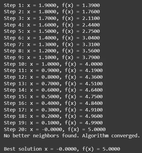
The output shows the successive values of x and f(x) as the algorithm moves toward the maximum, followed by the best solution (x=-0.0000, f(x)=5.0000) found.

You can download the source code from here.

Applications

• Pathfinding: Used to find good paths in robotics and games.
• Optimization: Helps solve scheduling, resource allocation, and other optimization problems.
• Game AI: Used to improve an AI's game position based on an evaluation function.
• Machine Learning: Can be used for tasks such as hyperparameter optimization.

Advantages

1. Low Memory Usage: Maintains only the current solution and its neighboring states, requiring little memory.
2. Fast Convergence: Can quickly reach a good solution when the search landscape provides a clear direction toward improvement.
3. Problem Independent: Can be applied to different optimization problems by defining a suitable objective function and neighborhood.
4. Easy to Customize: The neighborhood structure, evaluation function and stopping criteria can be adapted to the problem.

Limitations

1. Local Optima: May stop at a local maximum or minimum even when a better global solution exists.
2. Plateaus: Can get stuck in flat regions where neighboring states have the same evaluation value.
3. Ridges: Narrow or steep regions can make it difficult to find a direct improving move.
4. Initial State Dependence: Different starting states can lead to different solutions.
5. No Backtracking: Once the algorithm moves to a state, it generally does not revisit previous states, which can prevent it from escaping a poor region.