

Artificial Neural Networks (ANNs) are the fundamental building blocks of modern deep learning systems. They consist of interconnected artificial neurons organized into layers that learn from training data to recognize patterns, make predictions and solve complex problems.
- Organized into input, hidden and output layers
- Learn by adjusting weights and biases during training
- Process data through forward propagation and improve using backpropagation
- Support tasks such as classification, regression and prediction
- Form the foundation of advanced deep learning architectures such as CNNs, RNNs and Transformers
McCulloch-Pitts Model of Neuron
One of the earliest models of artificial neurons was the McCulloch-Pitts Model introduced in 1943. It is also known as the linear threshold gate.
- The neuron takes multiple inputs, each associated with a weight.
- A weighted sum of the inputs is calculated.
- If the weighted sum exceeds a threshold, the neuron fires (output = 1) otherwise it does not fire (output = 0).
Mathematically this is represented as:
f(y_{\text{in}}) = \begin{cases} 1, & \text{if } y_{\text{in}} \geq \Theta \\ 0, & \text{if } y_{\text{in}} < \Theta \end{cases}
where
y_{\text{in}} = \sum x_i w_i
This model laid the foundation for modern neural networks, though it is limited to solving only linearly separable problems.
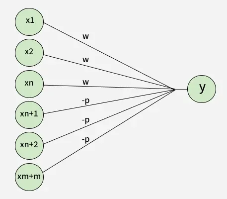
Artificial Neural Networks Algorithm
1. Initialize Weights and Bias
- The algorithm starts by initializing the weights i.e the strength of connections between neurons and biases which is additional parameters that help to adjust output.
- These values are usually initialized randomly.
- You also set the learning rate (α) which controls how much the weights should be adjusted during training.
2. Feed Input Data
The input data is fed into the input layer of the network. Each input is a feature like an image pixel, a value from a dataset, etc.
3. Forward Propagation (Calculate Output)
- The data is passed through the network from the input layer to the hidden layers and finally to the output layer.
- At each layer the input is multiplied by the weights and passed through an activation function like sigmoid, ReLU, etc to produce the output of that layer.
- The result is a prediction or an output that is compared to the actual target value.
4. Calculate Error
Once the network has made a prediction the next step is to calculate the error i.e the difference between the predicted output and the actual target. This error is often measured using a loss function like Mean Squared Error or Cross-Entropy.
5. Backpropagation (Update Weights)
Backpropagation computes the gradients i.e how much change in weights would reduce the error by using the chain rule of calculus. The weights and biases are then updated to minimize the error. The update is done using an optimization algorithm like Gradient Descent:
w = w - \alpha \times \frac{\partial \text{Error}}{\partial w}
6. Repeat (Epochs)
Steps 2 to 5 are repeated for multiple epochs which is iterations over the entire training dataset. During each epoch the weights are adjusted to reduce the error gradually.
7. Test the Network
After training, the network is tested with new data to evaluate its performance. If the accuracy is good, the training is considered complete. If not more training or adjustments may be needed.
How do Artificial Neural Networks learn?
Artificial Neural Networks learn by repeatedly improving their predictions from training examples. Consider the task of recognizing cats in images.
- The network is trained using thousands of labeled images of cats and non-cats.
- Each image passes through the network to generate a prediction.
- The predicted result is compared with the correct label to calculate the error.
- The network updates its weights and biases to reduce this error.
- This process is repeated over many training iterations until the network can accurately classify new images.
Common Activation Functions in ANNs
Activation functions are important in neural networks because they introduce non-linearity and helps the network to learn complex patterns. Lets see some common activation functions used in ANNs:
- Sigmoid Function: Outputs values between 0 and 1. It is used in binary classification tasks like deciding if an image is a cat or not.
- ReLU (Rectified Linear Unit): A popular choice for hidden layers, it returns the input if positive and zero otherwise. It helps to solve the vanishing gradient problem.
- Tanh (Hyperbolic Tangent): Similar to sigmoid but outputs values between -1 and 1. It is used in hidden layers when a broader range of outputs is needed.
- Softmax: Converts raw outputs into probabilities used in the final layer of a network for multi-class classification tasks.
- Leaky ReLU: A variant of ReLU that allows small negative values for inputs helps in preventing “dead neurons” during training.
These functions help the network decide whether to activate a neuron helps it to recognize patterns and make predictions.
For more details refer to Types of Activation Functions
Optimization Algorithms in ANN Training
Optimization algorithms adjust the weights of a neural network during training to minimize errors. The goal is to make the network’s predictions more accurate. Lets see key algorithms:
- Gradient Descent: Most basic optimization algorithm that updates weights by calculating the gradient of the loss function.
- Adam (Adaptive Moment Estimation): An efficient version of gradient descent that adapts learning rates for each weight used in deep learning.
- RMSprop: A variation of gradient descent that adjusts the learning rate based on the average of recent gradients, it is useful in training recurrent neural networks (RNNs).
- Stochastic Gradient Descent (SGD): Updates weights using one sample at a time helps in making it faster but more noisy.
For more details refer to Optimization Algorithms in ANN
Applications
- Classification: ANNs are widely used for tasks such as spam email detection, fraud detection, sentiment analysis, and customer churn prediction.
- Regression: They predict continuous values such as house prices, sales forecasts, stock trends, and energy consumption.
- Healthcare: ANNs assist in disease diagnosis, medical data analysis, and predicting patient health risks.
- Business and Recommendation Systems: They help recommend products, personalize user experiences, and analyze customer behavior for better decision-making.
Advantages
- Handle noisy and incomplete data without affecting their performance. Even if there are errors in the training data they can still produce accurate results.
- Once trained ANNs can evaluate functions very quickly making them ideal for real-time applications like self-driving cars or fraud detection.
- Handle large amounts of data through distributed processing similar to how the human brain works.
Limitations
- Can overfit to training data especially when the model is too complex or when there is insufficient data.
- Require large datasets for training to generalize well.
- Training deep neural networks can be computationally expensive and time-consuming hence requiring substantial hardware resources.
