

A learning curve is a graphical representation that shows how a model's performance changes as it learns from more data or training iterations. It helps evaluate whether a model is learning effectively and can be used to identify underfitting, overfitting or a well fitted model.
Understanding Learning Curve
A learning curve typically contains:
- Training Curve: Performance of the model on training data.
- Validation Curve: Performance of the model on unseen validation data.
- X-axis: Amount of training data or training iterations.
- Y-axis: Performance metric such as accuracy, error or loss.
Identifying Model Behaviour Using Learning Curves
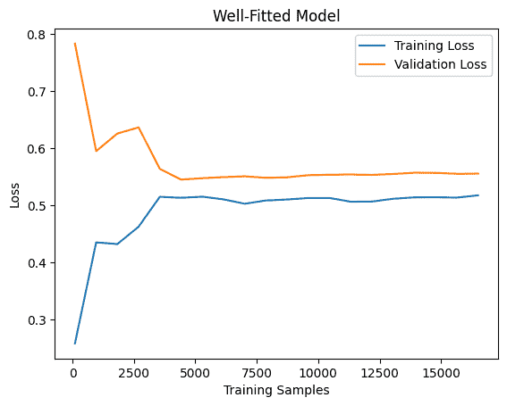
1. Well-Fitted Model
A well-fitted model learns the underlying patterns without memorizing the training data.
- Training and validation curves are close to each other.
- Both curves achieve good performance.
- Small gap between training and validation error.
- Good generalization to unseen data.
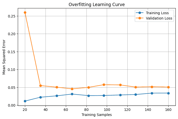
2. Overfitting
Overfitting occurs when a model learns the training data too well, including noise and irrelevant patterns. As a result, it performs well on training data but poorly on unseen data.
- Training error is very low.
- Validation error remains high.
- Large gap between training and validation curves.
- Poor generalization on new data.
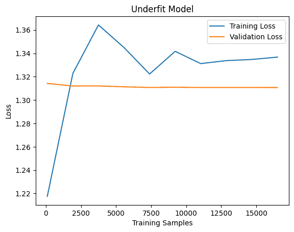
3. Underfitting
Underfitting occurs when the model is too simple to capture the underlying patterns in the data. It performs poorly on both training and validation datasets.
- High training error.
- High validation error.
- Both curves remain close but at poor performance levels.
- Model fails to learn important patterns.
Implementation
The following examples use the California Housing Dataset and Ridge Regression to generate learning curves and analyze model behavior.
1. Import Required Libraries
- Loads the California Housing dataset.
- Uses Ridge Regression as the learning model.
- Calculates prediction error using Mean Squared Error (MSE).
- Uses Matplotlib for visualization.
import numpy as np
import matplotlib.pyplot as plt

from sklearn.datasets import fetch_california_housing
from sklearn.linear_model import Ridge
from sklearn.model_selection import train_test_split
from sklearn.metrics import mean_squared_error
2. Load and Split Dataset
- Loads the dataset.
- Splits the data into training and validation sets.
- Validation data is used to evaluate model generalization.
data = fetch_california_housing()

X = data.data
y = data.target

X_train, X_val, y_train, y_val = train_test_split(
    X,
    y,
    test_size=0.2,
    random_state=42
)
3. Learning Curve of a Well-Fitted Model
- Trains Ridge Regression on increasing amounts of data.
- Calculates training and validation loss.
- A small gap between both curves indicates a well-fitted model.
train_loss = []
val_loss = []

sizes = np.linspace(
    100,
    len(X_train),
    20,
    dtype=int
)

for size in sizes:

    model = Ridge(alpha=1.0)

    model.fit(
        X_train[:size],
        y_train[:size]
    )

    train_pred = model.predict(
        X_train[:size]
    )

    val_pred = model.predict(
        X_val
    )

    train_loss.append(
        mean_squared_error(
            y_train[:size],
            train_pred
        )
    )

    val_loss.append(
        mean_squared_error(
            y_val,
            val_pred
        )
    )

plt.plot(
    sizes,
    train_loss,
    label="Training Loss"
)

plt.plot(
    sizes,
    val_loss,
    label="Validation Loss"
)

plt.title("Well-Fitted Model")
plt.xlabel("Training Samples")
plt.ylabel("Loss")
plt.legend()
plt.show()
Output:
4. Learning Curve of an Overfit Model
- Uses a high-degree polynomial model.
- Training loss becomes very low.
- Validation loss remains high.
import numpy as np
import matplotlib.pyplot as plt

from sklearn.model_selection import train_test_split
from sklearn.preprocessing import PolynomialFeatures
from sklearn.linear_model import LinearRegression
from sklearn.metrics import mean_squared_error

np.random.seed(42)

X = np.random.rand(200, 1) * 10
y = np.sin(X).ravel() + np.random.normal(0, 0.2, 200)

X_train, X_val, y_train, y_val = train_test_split(
    X,
    y,
    test_size=0.2,
    random_state=42
)

train_loss = []
val_loss = []

sizes = np.linspace(20, len(X_train), 10, dtype=int)

for size in sizes:

    poly = PolynomialFeatures(degree=10)

    X_train_poly = poly.fit_transform(X_train[:size])
    X_val_poly = poly.transform(X_val)

    model = LinearRegression()

    model.fit(X_train_poly, y_train[:size])

    train_pred = model.predict(X_train_poly)
    val_pred = model.predict(X_val_poly)

    train_loss.append(
        mean_squared_error(
            y_train[:size],
            train_pred
        )
    )

    val_loss.append(
        mean_squared_error(
            y_val,
            val_pred
        )
    )

plt.figure(figsize=(8,5))

plt.plot(
    sizes,
    train_loss,
    marker='o',
    label='Training Loss'
)

plt.plot(
    sizes,
    val_loss,
    marker='o',
    label='Validation Loss'
)

plt.title("Overfitting Learning Curve")
plt.xlabel("Training Samples")
plt.ylabel("Mean Squared Error")

plt.legend()
plt.grid(True)

plt.show()
Output:
5. Learning Curve of an Underfit Model
- Uses a very simple model that predicts the mean value.
- Both training and validation losses remain high.
- Indicates that the model is unable to learn meaningful patterns.
from sklearn.dummy import DummyRegressor

train_loss = []
val_loss = []

for size in sizes:

    model = DummyRegressor(
        strategy="mean"
    )

    model.fit(
        X_train[:size],
        y_train[:size]
    )

    train_pred = model.predict(
        X_train[:size]
    )

    val_pred = model.predict(
        X_val
    )

    train_loss.append(
        mean_squared_error(
            y_train[:size],
            train_pred
        )
    )

    val_loss.append(
        mean_squared_error(
            y_val,
            val_pred
        )
    )

plt.plot(
    sizes,
    train_loss,
    label="Training Loss"
)

plt.plot(
    sizes,
    val_loss,
    label="Validation Loss"
)

plt.title("Underfit Model")
plt.xlabel("Training Samples")
plt.ylabel("Loss")
plt.legend()
plt.show()
Output:
Download full code from here
