

The Chi-Square test is a statistical method used to determine if there is a significant association between categorical variables. When dealing with multiple columns, you can use Chi-Square tests to explore relationships across several categorical variables simultaneously. In this article, we’ll go through the steps to conduct Chi-Square tests for multiple columns in R, including data preparation, executing the tests, and interpreting the results using R Programming Language.
Understanding the Chi-Square Test
The Chi-Square test examines whether the distribution of categorical variables differs from what would be expected by chance. It is often used in two primary forms:
- Chi-Square Test of Independence: Tests whether two categorical variables are independent.
- Chi-Square Goodness of Fit Test: Tests whether the observed frequencies match expected frequencies.
Now we will discuss step by step implementation of Chi-Square Tests for Multiple Columns in R.
Step 1: Install and Load Required Packages
For conducting Chi-Square tests, we can use base R functions. However, it's beneficial to have dplyr and ggplot2 for data manipulation and visualization.
install.packages("dplyr")
install.packages("ggplot2")

library(dplyr)
library(ggplot2)
Step 2: Create a Sample Dataset
Let’s create a sample dataset that contains multiple categorical variables.
# Create a sample dataset
set.seed(123)
data <- data.frame(
  Gender = sample(c("Male", "Female"), 100, replace = TRUE),
  Preference = sample(c("Product A", "Product B", "Product C"), 100, replace = TRUE),
  AgeGroup = sample(c("Young", "Middle-aged", "Old"), 100, replace = TRUE)
)

# View the first few rows of the dataset
head(data)
Output:
  Gender Preference    AgeGroup
1   Male  Product A       Young
2   Male  Product B Middle-aged
3   Male  Product A       Young
4 Female  Product B         Old
5   Male  Product A       Young
6 Female  Product C       Young
Step 3: Create Contingency Tables
To perform Chi-Square tests, you need to create contingency tables that summarize the frequencies of the categorical variables.
# Create contingency tables
contingency_table_gender_pref <- table(data$Gender, data$Preference)
contingency_table_gender_age <- table(data$Gender, data$AgeGroup)
contingency_table_pref_age <- table(data$Preference, data$AgeGroup)

# View contingency tables
contingency_table_gender_pref
contingency_table_gender_age
contingency_table_pref_age
Output:
         Product A Product B Product C
  Female        12        18        13
  Male          14        21        22


         Middle-aged Old Young
  Female          15   6    22
  Male            13  17    27


            Middle-aged Old Young
  Product A           4   6    16
  Product B          10  12    17
  Product C          14   5    16
Step 4: Perform Chi-Square Tests
Now we can conduct Chi-Square tests for each of the contingency tables we created.
# Perform Chi-Square tests
chi_square_gender_pref <- chisq.test(contingency_table_gender_pref)
chi_square_gender_age <- chisq.test(contingency_table_gender_age)
chi_square_pref_age <- chisq.test(contingency_table_pref_age)

# View the results
chi_square_gender_pref
chi_square_gender_age
chi_square_pref_age
Output:
	Pearson's Chi-squared test

data:  contingency_table_gender_pref
X-squared = 0.75367, df = 2, p-value = 0.686


	Pearson's Chi-squared test

data:  contingency_table_gender_age
X-squared = 4.033, df = 2, p-value = 0.1331


	Pearson's Chi-squared test

data:  contingency_table_pref_age
X-squared = 6.6788, df = 4, p-value = 0.1539
The output of the chisq.test() function includes:
- X-squared: The test statistic.
- df: Degrees of freedom.
- p-value: The probability of observing the data if the null hypothesis is true.
A low p-value (typically < 0.05) indicates that you can reject the null hypothesis, suggesting that there is an association between the variables.
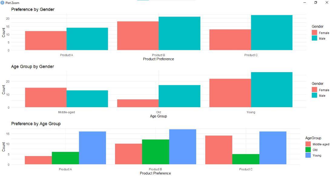
Step 6: Visualize the Results
Visualizations can help to better understand the associations between categorical variables. Here’s how to create bar plots to visualize the counts in contingency tables.
library(dplyr)
library(ggplot2)
library(gridExtra)


# Bar plot for Gender and Preference
plot_gender_pref <- ggplot(data, aes(x = Preference, fill = Gender)) +
  geom_bar(position = "dodge") +
  labs(title = "Preference by Gender",
       x = "Product Preference",
       y = "Count") +
  theme_minimal()

# Bar plot for Gender and Age Group
plot_gender_age <- ggplot(data, aes(x = AgeGroup, fill = Gender)) +
  geom_bar(position = "dodge") +
  labs(title = "Age Group by Gender",
       x = "Age Group",
       y = "Count") +
  theme_minimal()

# Bar plot for Preference and Age Group
plot_pref_age <- ggplot(data, aes(x = Preference, fill = AgeGroup)) +
  geom_bar(position = "dodge") +
  labs(title = "Preference by Age Group",
       x = "Product Preference",
       y = "Count") +
  theme_minimal()

# Arrange the plots in a grid layout
grid.arrange(plot_gender_pref, plot_gender_age, plot_pref_age, ncol = 1)
Output:
Conclusion
Conducting Chi-Square tests for multiple columns in R allows you to explore relationships between categorical variables effectively. By following the steps outlined in this article, you can create contingency tables, perform Chi-Square tests, interpret the results, and visualize the findings. This approach is essential for understanding the dynamics of categorical data and drawing meaningful insights from it.
