How to Visualize Kurtosis in R

Kurtosis is a statistical measure that describes the shape of a distribution's tails about its overall shape. It indicates how heavy or light the tails of a distribution are compared to a normal distribution. In this article, we will learn how to calculate and visualize kurtosis in R.

Why Visualizing Kurtosis is Important

Visualizing kurtosis is essential because it helps you understand the shape and distribution characteristics of your data, particularly the tails and peaks of the distribution. Kurtosis measures the extent to which data points in a distribution have extreme values (outliers), and a visual representation makes it easier to comprehend these statistical nuances.

Now we will discuss step by step How to Visualize Kurtosis in R Programming Language:

Step 1: Installing Required Packages

To calculate and visualize kurtosis in R, we will use several libraries, including moments for statistical calculations and ggplot2 for visualizations. Make sure you have these packages installed:

install.packages("moments")    # For kurtosis calculation
install.packages("ggplot2")    # For visualization
install.packages("dplyr")      # For data manipulation

Step 2: Calculating Kurtosis in R

We can calculate kurtosis using the kurtosis() function from the moments package. Let’s generate a simple random dataset to demonstrate how to compute kurtosis.

# Load required libraries
library(moments)
library(ggplot2)

# Generate a random normal dataset
set.seed(123)
data <- rnorm(1000, mean = 0, sd = 1)

# Calculate kurtosis
kurt_value <- kurtosis(data)
kurt_value

Output:

[1] 2.925747

Here, kurt_value will give us the kurtosis of the dataset. Since we generated a normal distribution, the kurtosis should be close to 3 (mesokurtic).

Step 3: Visualizing Distribution with ggplot2

Visualizing the distribution is essential to understanding kurtosis. We will use a histogram and overlay a density curve to visualize the shape of the data distribution.

# Create a histogram with density plot
ggplot(data.frame(data), aes(x = data)) +
  geom_histogram(aes(y = ..density..), bins = 30, fill = "lightblue", color = "black", alpha = 0.7) +
  geom_density(color = "red", size = 1.2) +
  labs(title = "Histogram with Density Curve", x = "Values", y = "Density") +
  theme_minimal()

Output:

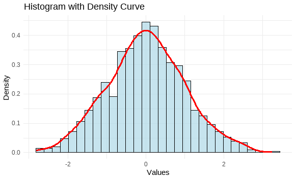
The histogram with the density curve will allow us to visually inspect the peak and tails of the distribution, which are indicative of kurtosis.

Step 4: Comparing Distributions with Different Kurtosis

To understand kurtosis better, let’s compare a normal distribution (mesokurtic) with distributions that have higher (leptokurtic) and lower (platykurtic) kurtosis.

# Generate datasets with different kurtosis levels
data_leptokurtic <- c(rnorm(900, mean = 0, sd = 1), rnorm(100, mean = 0, sd = 5)) # Heavy-tailed
data_platykurtic <- runif(1000, min = -2, max = 2)  # Uniform distribution

# Calculate kurtosis for each dataset
kurt_leptokurtic <- kurtosis(data_leptokurtic)
kurt_platykurtic <- kurtosis(data_platykurtic)

# Print kurtosis values
cat("Leptokurtic Kurtosis:", kurt_leptokurtic, "\n")
cat("Platykurtic Kurtosis:", kurt_platykurtic, "\n")

# Create combined dataframe
data_combined <- data.frame(
  values = c(data, data_leptokurtic, data_platykurtic),
  type = rep(c("Normal", "Leptokurtic", "Platykurtic"), each = 1000)
)

# Visualize the different distributions
ggplot(data_combined, aes(x = values, fill = type)) +
  geom_histogram(aes(y = ..density..), bins = 30, color = "black", alpha = 0.6) +
  geom_density(aes(color = type), size = 1.2) +
  facet_wrap(~ type, scales = "free") +
  labs(title = "Comparison of Distributions with Different Kurtosis",
       x = "Values", y = "Density") +
  theme_minimal()

Output:

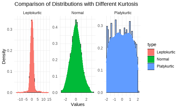
• High Kurtosis (Leptokurtic): A kurtosis value greater than 3 indicates a distribution with heavy tails and a sharp peak. This suggests the presence of more extreme values or outliers.
• Low Kurtosis (Platykurtic): A kurtosis value less than 3 indicates a distribution with lighter tails and a flatter peak. This suggests fewer extreme values.
• Normal Kurtosis (Mesokurtic): A kurtosis value of approximately 3 is typical of a normal distribution, which has moderate tails and a well-proportioned peak.

Real-World Data Example

Let's visualize the kurtosis of a real-world dataset, such as the mtcars dataset. We will calculate and visualize the kurtosis of the "mpg" (miles per gallon) variable.

# Load mtcars dataset
data("mtcars")

# Calculate kurtosis for mpg
kurt_mpg <- kurtosis(mtcars$mpg)
kurt_mpg

# Plot histogram and density of mpg
ggplot(mtcars, aes(x = mpg)) +
  geom_histogram(aes(y = ..density..), bins = 10, fill = "lightgreen", color = "black", alpha = 0.7) +
  geom_density(color = "blue", size = 1.2) +
  labs(title = "MPG Distribution with Density Curve", x = "Miles Per Gallon", y = "Density") +
  theme_minimal()

Output:

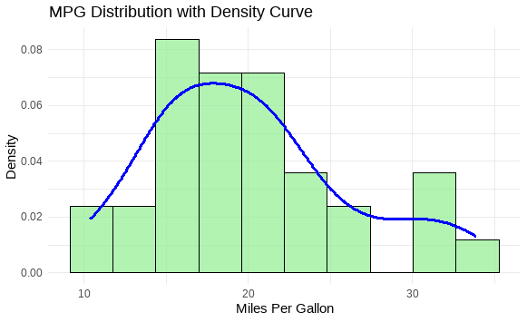
The kurtosis value of "mpg" will give insights into whether the distribution of miles per gallon in the dataset has a sharp peak or heavy tails.

Conclusion

Kurtosis is a useful statistical measure for understanding the shape of a data distribution, especially its tails and peak. In this article, we demonstrated how to calculate and visualize kurtosis in R using the moments package for statistical calculations and ggplot2 for visualizations. By comparing different types of distributions (mesokurtic, leptokurtic, and platykurtic), we gained a clearer understanding of how kurtosis affects the shape of the data. Whether you are analyzing financial data, biological measurements, or any dataset, understanding kurtosis can help you assess the likelihood of extreme outcomes and the overall distribution characteristics.