Partial Autocorrelation Function in R

In time series analysis, understanding the relationships between data points over time is crucial for making accurate predictions and informed decisions. One of the key tools in this analysis is the Partial Autocorrelation Function (PACF). PACF helps us gauge how current observations in a time series relate to past observations while controlling for the influence of intervening values. This article clears the concept of PACF, its importance in modeling, and practical implementations using R.

What is Partial Autocorrelation?

Partial Autocorrelation measures the correlation between the observations at the time t and t-k, but after removing the effects of the values in between (e.g., at time t-1, t-2, …, t-(k-1)). It's particularly useful when building autoregressive (AR) models because it helps identify the order of the model (the number of lags to include).

Formula:

[ PACF(k) = \frac{ACF(k) - \sum_{j=1}^{k-1} PACF(j) \cdot ACF(k-j)}{1 - \sum_{j=1}^{k-1} PACF(j) \cdot ACF(j)} ]

Here,

• ACF(k) is the autocorrelation function at lag k.
• ∑ j=1k−1 : Summation term used to adjust for the effects of earlier lags.

Importance of PACF in Time Series Analysis

• Identifying the Order of AR Models: PACF can indicate the number of lagged terms to include in an autoregressive model.
• Model Selection: By analyzing PACF plots, analysts can determine the appropriate parameters for ARIMA models, facilitating effective forecasting.
• Understanding Relationships: PACF provides insights into the direct dependencies between data points at various lags, which can be invaluable for interpretation.

Difference Between ACF and PACF

Now we implement Partial Autocorrelation Function in Time Series Using R Programming Language.

Step 1: Install and Load Required Libraries

First, install and load the necessary libraries.

# Install necessary packages if not already installed
install.packages("forecast")   # For PACF function
install.packages("ggplot2")    # For visualization (optional)

# Load the libraries
library(forecast)
library(ggplot2)

Step 2: Load the Dataset

Now load the dataset and check first few rows.

# Load the dataset
data("AirPassengers")

# View the first few rows
head(AirPassengers)

Output:

     Jan Feb Mar Apr May Jun
1949 112 118 132 129 121 135

Step 3: Visualization

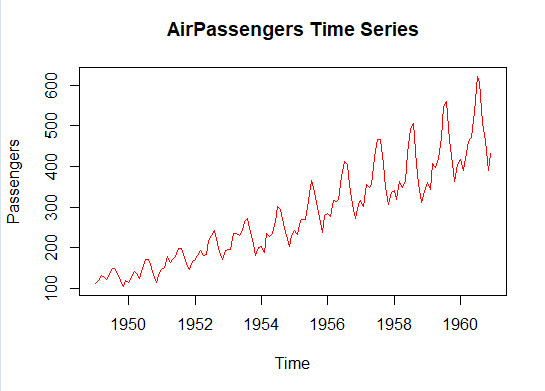
To visualize the data, we can plot the time series.

plot(ts_data, main = "AirPassengers Time Series", ylab = "Passengers", xlab = "Time" , col="red")

Output:

Step 4: Test for Stationarity

Before performing PACF or fitting an ARIMA model, we need to check whether the series is stationary.

# Perform the Augmented Dickey-Fuller (ADF) test for stationarity
adf_test <- adf.test(AirPassengers)

# Print the results of the ADF test
print(adf_test)

Output:

	Augmented Dickey-Fuller Test

data:  AirPassengers
Dickey-Fuller = -7, Lag order = 5, p-value = 0.01
alternative hypothesis: stationary

If the p-value is greater than 0.05, the series is non-stationary, meaning it has trends or seasonality and needs differencing.

Step 5: Calculate and Plot Partial Autocorrelation (PACF)

Now, to compute and plot the partial autocorrelation, use the pacf() function.

# PACF plot
pacf(air_passengers, main="Partial Autocorrelation of Air Passengers" , col="hotpink")

Output:

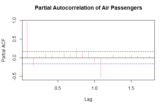
Here, A sharp cutoff after a few lags indicates the appropriate lag order for an autoregressive (AR) model. For example, if the PACF plot shows significant correlations only up to lag 1 or 2, you might consider an AR(1) or AR(2) model.

Step 6: Build a Model

Now build a ARIMA Model from PACF.

# Build ARIMA model based on PACF plot
# ARIMA(2,1,0) suggests 2 AR terms, first-order differencing, and no MA terms
model <- Arima(AirPassengers, order=c(2,1,0))

# Display the summary of the ARIMA model
summary(model)

Output:

Series: AirPassengers 
ARIMA(2,1,0) 

Coefficients:
        ar1     ar2
      0.381  -0.228
s.e.  0.082   0.083

sigma^2 = 991:  log likelihood = -695
AIC=1397   AICc=1397   BIC=1405

Training set error measures:
               ME RMSE  MAE   MPE MAPE  MASE   ACF1
Training set 2.04 31.2 24.5 0.416 8.68 0.764 -0.036

Step 7: Perform Model Diagnostics

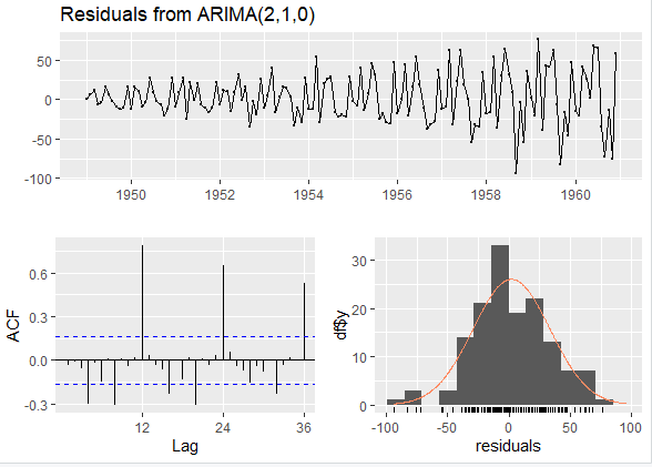
Next, we need to check the residuals to ensure that the model is adequate.

# Check the residuals to ensure the model is adequate
checkresiduals(model)

# Perform Ljung-Box test to check residual autocorrelation
Box.test(residuals(model), type="Ljung-Box")

Output:

	Ljung-Box test

data:  Residuals from ARIMA(2,1,0)
Q* = 235, df = 22, p-value <2e-16

Model df: 2.   Total lags used: 24


	Box-Ljung test

data:  residuals(model)
X-squared = 0.2, df = 1, p-value = 0.7

Plot the Value,

Step 8: Plot the Forecasted Values

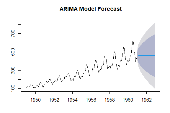
Now forecast the future values.

# Forecast the next 24 months based on the fitted ARIMA model
forecast_values <- forecast(model, h=24)

# Plot the forecasted values
plot(forecast_values, main="ARIMA Model Forecast")

Output:

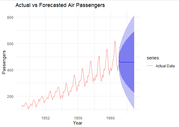
Step 9: Visualize Actual vs Forecasted Values

Now compare the actual vs forecasted values.

# Plot actual vs forecasted values
autoplot(forecast_values) + 
  autolayer(AirPassengers, series="Actual Data") +
  ggtitle("Actual vs Forecasted Air Passengers") +
  xlab("Year") + ylab("Passengers") +
  theme_minimal()

Output:

Applications of PACF

• Time Series Forecasting: PACF helps identify AR components, essential for ARIMA models, allowing accurate predictions of future values.
• Financial Market Analysis: PACF can determine patterns in stock prices, including trends and seasonal fluctuations.
• Sales Forecasting: It aids in predicting sales trends and identifying seasonal demand variations.
• Weather Analysis: Useful for analyzing temperature, rainfall, and other meteorological patterns over time.
• Anomaly Detection: Identifying unusual events or outliers in time series data by detecting deviations from expected patterns.

Best Practices for Using PACF

• Minor spikes in the PACF plot may not indicate significant relationships. Focus on pronounced spikes beyond the confidence intervals.
• PACF is most effective when the time series is stationary. If the data exhibits strong trends or seasonality, consider differencing or applying transformations before analysis.
• For data with seasonality, seasonal ARIMA models (SARIMA) may be more suitable.

Conclusion

The Partial Autocorrelation Function (PACF) is a vital tool in time series analysis, providing valuable insights into the direct relationships between past and present values. By interpreting PACF plots, analysts can make informed decisions regarding model selection and forecasting. In combination with other tools like the Autocorrelation Function (ACF), PACF enhances our ability to understand and model complex time series data effectively.